Retention Times Match Factor - Unknowns Analysis

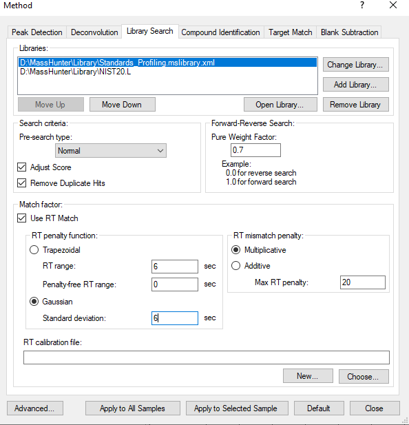
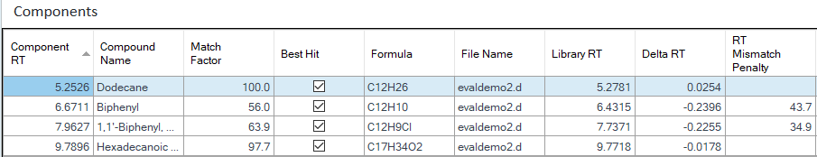
Hello, I am using an Agilent 8890 GC with a 7000D triple quadrupole. I have MassHunter version 10.0 with Quant and Qual software. I am trying to optimize library and compound identification parameters in the Unknowns Analysis Program and Qualitative Analysis program. Specifically I am confused on the RT Match settings. I don't understand the meaning of some of these settings. I don't understand the difference between the RT penalty functions and RT mismatch penalty. 

Basically what I want library to do is search my custom user library using RT and spectra. If RT is outside a certain window (5 seconds, 10 seconds, 30 seconds whatever) I want to reject that hit and with NIST. If I ignore RT what happens is my custom library ends up finding the same compounds at multiple retention times which I know are wrong. So I want to use RT to reject these incorrect hits and use NIST to give me an idea what they might be. But these settings are new to me and I can't find clear explanation what they mean in any of the manuals / webinars I've looked at. 

Parents
  • Hello  ,

    An interesting question. While there is information on these settings in the Qual help file and in the Unknowns Analysis Data Set manual, there are not many good examples or explanations of how the settings are used. So let me try to explain.

    First, the short answer.

    If you just want to set a fixed RT window and have a match either be accepted if it is in that range or rejected if it is not, choose Trapezoidal, set RT range and Penalty-free RT range to the same value, and set the RT mismatch penalty to Multiplicative. Any compound that is within the RT range will not have a penalty applied for its retention time and will only use the Library Match Factor to determine its score. Any compound not within that RT range will have its match score set to 0 and be rejected.

    Now for the gory details, with at least a few pictures to help break the wall of words.

    The RT Penalty function calculates a value from 1 to 0 based on the delta RT. This is set to 1 if there is a perfect RT match, 0 if it falls outside of the criteria as determined by the penalty function settings, or a fractional value depending on the shape of the penalty function curve used. The penalty function is then applied according to the RT mismatch penalty such that a score of 1 will apply no penalty, a score of 0 will apply the full penalty, and any value in between will apply a fractional penalty.

    There are two options for calculating the RT penalty function. The trapezoidal penalty function will use an isosceles trapezoidal 'curve' to calculate the value of the penalty. Delta RTs that fall within the Penalty-free RT range will have no penalty applied for the RT match. Any delta RT between the Penalty-free range and the RT range will have a fractional value calculated using the sides of the trapezoid. Any delta RT outside of the RT range will receive the full RT penalty.

    Here is a graphical representation from the Data Set manual -

    Example - If the RT range is set to 10 seconds and the Penalty-free RT range is set to 5, if a compound has a delta RT of 4 seconds there will be no penalty applied. If the delta RT is 6 seconds then the penalty function will be 0.8. If the delta RT is 11 seconds then the full penalty is applied.

    If the RT range and Penalty-free RT range are equal, then you are using a rectangle and you end up with the simple case from my short version of the answer. Here is a graphical representation from the Data Set manual - 

    The Gaussian works in the same way, there is just a bit more math involved.

    Here is a graphical representation from the Data Set manual -

    Basically, as the delta RT increases the penalty function will decrease following the gaussian distribution curve. The setting for Standard Deviation determines the width of the curve. This method is far less forgiving than trapezoidal and more difficult to visualize, at least for me.

    So, moving quickly on...

    The RT Mismatch Penalty determines how the value of the RT Penalty Function is applied to the Library Match Factor.

    The Multiplicative penalty simply multiplies the Library Match Score by the RT Penalty Function.

    Library Match Score = Library Match Factor * RT Penalty function

    So, a penalty of 1 makes no change (perfect RT match), a penalty of 0 makes the score 0 (completely outside the RT range), and anything in between reduces the match score by that fractional amount. For example, a resulting penalty of 0.5 would cut the Library Match Score in half, taking a score of 90 down to 45.

    The Additive penalty allows you to set a Max RT penalty. This would ensure that even if the RT Penalty Function is 0, the match is not completely disregarded.

    Library Match Score = Library Match Factor – MaxRTPenalty * (1 – RT Penalty Function)

    So here a penalty of 0 would not make the match score 0 as it would with Multiplicative, but only penalize the score by the maximum penalty. A perfect score of 1 would result in 0 being subtracted from the match factor, and again anything in between would apply the resulting fractional penalty.

    For added fun, you can show the RT Mismatch Penalty column in your UA results table to see how big of a hit you are taking for a given delta RT. This was a 10 second penalty free trapezoid with a 20 second window, just to show how it works.

Reply
  • Hello  ,

    An interesting question. While there is information on these settings in the Qual help file and in the Unknowns Analysis Data Set manual, there are not many good examples or explanations of how the settings are used. So let me try to explain.

    First, the short answer.

    If you just want to set a fixed RT window and have a match either be accepted if it is in that range or rejected if it is not, choose Trapezoidal, set RT range and Penalty-free RT range to the same value, and set the RT mismatch penalty to Multiplicative. Any compound that is within the RT range will not have a penalty applied for its retention time and will only use the Library Match Factor to determine its score. Any compound not within that RT range will have its match score set to 0 and be rejected.

    Now for the gory details, with at least a few pictures to help break the wall of words.

    The RT Penalty function calculates a value from 1 to 0 based on the delta RT. This is set to 1 if there is a perfect RT match, 0 if it falls outside of the criteria as determined by the penalty function settings, or a fractional value depending on the shape of the penalty function curve used. The penalty function is then applied according to the RT mismatch penalty such that a score of 1 will apply no penalty, a score of 0 will apply the full penalty, and any value in between will apply a fractional penalty.

    There are two options for calculating the RT penalty function. The trapezoidal penalty function will use an isosceles trapezoidal 'curve' to calculate the value of the penalty. Delta RTs that fall within the Penalty-free RT range will have no penalty applied for the RT match. Any delta RT between the Penalty-free range and the RT range will have a fractional value calculated using the sides of the trapezoid. Any delta RT outside of the RT range will receive the full RT penalty.

    Here is a graphical representation from the Data Set manual -

    Example - If the RT range is set to 10 seconds and the Penalty-free RT range is set to 5, if a compound has a delta RT of 4 seconds there will be no penalty applied. If the delta RT is 6 seconds then the penalty function will be 0.8. If the delta RT is 11 seconds then the full penalty is applied.

    If the RT range and Penalty-free RT range are equal, then you are using a rectangle and you end up with the simple case from my short version of the answer. Here is a graphical representation from the Data Set manual - 

    The Gaussian works in the same way, there is just a bit more math involved.

    Here is a graphical representation from the Data Set manual -

    Basically, as the delta RT increases the penalty function will decrease following the gaussian distribution curve. The setting for Standard Deviation determines the width of the curve. This method is far less forgiving than trapezoidal and more difficult to visualize, at least for me.

    So, moving quickly on...

    The RT Mismatch Penalty determines how the value of the RT Penalty Function is applied to the Library Match Factor.

    The Multiplicative penalty simply multiplies the Library Match Score by the RT Penalty Function.

    Library Match Score = Library Match Factor * RT Penalty function

    So, a penalty of 1 makes no change (perfect RT match), a penalty of 0 makes the score 0 (completely outside the RT range), and anything in between reduces the match score by that fractional amount. For example, a resulting penalty of 0.5 would cut the Library Match Score in half, taking a score of 90 down to 45.

    The Additive penalty allows you to set a Max RT penalty. This would ensure that even if the RT Penalty Function is 0, the match is not completely disregarded.

    Library Match Score = Library Match Factor – MaxRTPenalty * (1 – RT Penalty Function)

    So here a penalty of 0 would not make the match score 0 as it would with Multiplicative, but only penalize the score by the maximum penalty. A perfect score of 1 would result in 0 being subtracted from the match factor, and again anything in between would apply the resulting fractional penalty.

    For added fun, you can show the RT Mismatch Penalty column in your UA results table to see how big of a hit you are taking for a given delta RT. This was a 10 second penalty free trapezoid with a 20 second window, just to show how it works.

Children
Was this helpful?